Privacy Preserving k-means¶

Data privacy is an extremely sensitive topic which requires a selection of methods/techniques when processing or using individuals data. Some new approaches to this involve the creation of synthetic data or the move away from sharing any individuals data at all to a single central data source. This second approach involves processing data at source and sharing only the key information centrally. This can mean processing data within a device, or at a central source (i.e. within a single study) and then sharing only the key information that is needed about that data. This section will discuss how information could be shared in this case between studies to gain a central cluster without passing on any individuals data from one study to another.

import pandas as pd
import numpy as np
from sklearn.preprocessing import OneHotEncoder
from sklearn.preprocessing import LabelEncoder
from sklearn import preprocessing
import matplotlib
import seaborn as sns
import matplotlib.pyplot as plt
from sklearn.cluster import KMeans
from sklearn.metrics import silhouette_score
from sklearn.decomposition import PCA
from matplotlib.pyplot import figure
import array

data = pd.read_csv('../data/cleaned_data.csv')

data

	Unnamed: 0	index	Deck_A	Deck_B	Deck_C	Deck_D	tot_win	tot_los	Subj	Study	Unique_ID	balance	Payoff
0	0	Subj_1	12	9	3	71	5800	-4650	1	Fridberg	1	1150	1
1	1	Subj_2	24	26	12	33	7250	-7925	2	Fridberg	2	-675	1
2	2	Subj_3	12	35	10	38	7100	-7850	3	Fridberg	3	-750	1
3	3	Subj_4	11	34	12	38	7000	-7525	4	Fridberg	4	-525	1
4	4	Subj_5	10	24	15	46	6450	-6350	5	Fridberg	5	100	1
...	...	...	...	...	...	...	...	...	...	...	...	...	...
612	93	Subj_94	24	69	13	44	12150	-11850	94	Wetzels	613	300	2
613	94	Subj_95	5	31	46	68	9300	-7150	95	Wetzels	614	2150	2
614	95	Subj_96	18	19	37	76	9350	-7900	96	Wetzels	615	1450	2
615	96	Subj_97	25	30	44	51	10250	-9050	97	Wetzels	616	1200	2
616	97	Subj_98	11	104	6	29	13250	-15050	98	Wetzels	617	-1800	2

617 rows × 13 columns

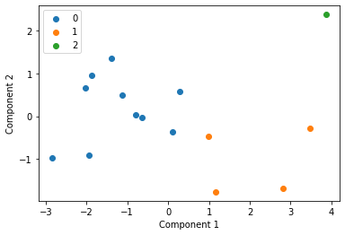
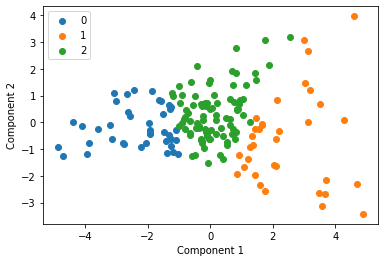
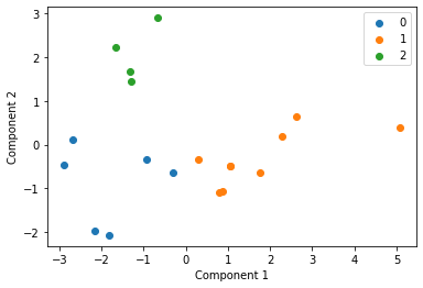
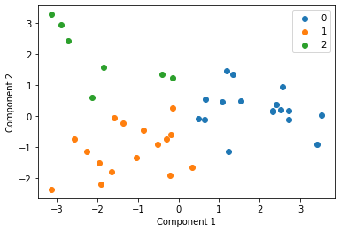
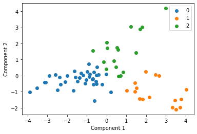
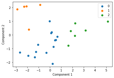
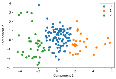
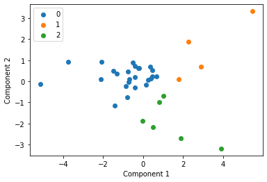
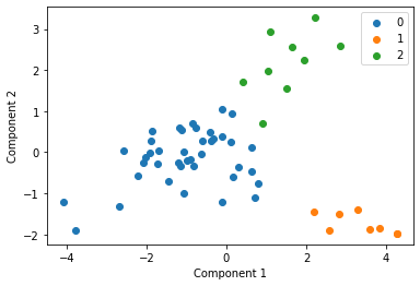
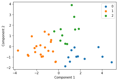
Clustering by study¶

We cluster each study individually with k=3 and display these clusters below

Fridberg = data[data['Study']=='Fridberg']
Horstmann = data[data['Study']=='Horstmann']
Kjome = data[data['Study']=='Kjome']
Maia = data[data['Study']=='Maia']
SteingroverInPrep = data[data['Study']=='SteingroverInPrep']
Premkumar = data[data['Study']=='Premkumar']
Wood = data[data['Study']=='Wood']
Worthy = data[data['Study']=='Worthy']
Steingroever2011 = data[data['Study']=='Steingroever2011']
Wetzels = data[data['Study']=='Wetzels']

l = [Fridberg, Horstmann, Kjome, Maia, SteingroverInPrep, Premkumar, Wood, Worthy, Steingroever2011, Wetzels]

clusters = []
labels = []
for s in l:
    df = s.drop(columns=['index', 'Subj', 'Study', 'Unnamed: 0', 'Unique_ID', 'balance'])

    scaler = preprocessing.StandardScaler().fit(df)
    X_scaled = scaler.transform(df)

    #rename columns to clearly represent decks
    sd = pd.DataFrame(X_scaled, columns=['Deck_1', 'Deck_2', 'Deck_3', 'Deck_4', 'tot_win', 'tot_los', 'Payoff'])
    sd

    pca = PCA(2)
    df = pca.fit_transform(sd)

    #w_out = pd.DataFrame(df, columns=['Component_1', 'Component_2'])
    #w_out_payoff = sd.drop(columns=["Payoff"])

    #w_out = pca.fit_transform(w_out_payoff)

    kmeans = KMeans(n_clusters= 3)
 
    #predict the labels of clusters.
    label = kmeans.fit_predict(df)
    for v in label:
        labels.append(v)
 
    #Getting unique labels
    u_labels = np.unique(label)

    centroids = kmeans.cluster_centers_
    clusters.append(centroids)
    
    #plotting the results:
    for i in u_labels:
        plt.scatter(df[label == i , 0] , df[label == i , 1] , label = i)
    plt.legend()
    plt.xlabel("Component 1")
    plt.ylabel("Component 2")
    plt.show()

../_images/Privacy_preserving_k_means_6_0.png

../_images/Privacy_preserving_k_means_6_1.png

../_images/Privacy_preserving_k_means_6_2.png

../_images/Privacy_preserving_k_means_6_3.png

../_images/Privacy_preserving_k_means_6_4.png

../_images/Privacy_preserving_k_means_6_5.png

../_images/Privacy_preserving_k_means_6_6.png

../_images/Privacy_preserving_k_means_6_7.png

../_images/Privacy_preserving_k_means_6_8.png

../_images/Privacy_preserving_k_means_6_9.png

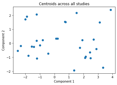
Centroid collection¶

We make a list called clusters above, with all of the centroids for each of the studies and plot these all together in the next cell. This gives an indication of each studies data distribution without providing any raw data centrally.

arr = np.vstack(clusters)
plt.scatter(arr[:,0], arr[:,1])
plt.title("Centroids across all studies")
plt.xlabel("Component 1")
plt.ylabel("Component 2")
plt.show()

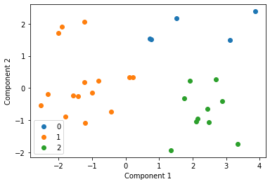
../_images/Privacy_preserving_k_means_8_0.png

Final clustering¶

We then cluster these centroids to see what our final distribution is like

kmeans = KMeans(n_clusters= 3)
 
#predict the labels of clusters.
label = kmeans.fit_predict(arr)
 
#Getting unique labels
u_labels = np.unique(label)

    
#plotting the results:
for i in u_labels:
    plt.scatter(arr[label == i , 0] , arr[label == i , 1] , label = i)
plt.legend()
#plt.title()
plt.xlabel("Component 1")
plt.ylabel("Component 2")
plt.show()
 

../_images/Privacy_preserving_k_means_10_0.png

CA4015 - Clustering Analysis of the Iowa Gambling Task

Privacy Preserving k-means¶

Clustering by study¶

Centroid collection¶

Final clustering¶

Analysis¶