Data Cleaning¶

We load in the relevant files for inspection and carry out a number of data manipulations, visualisations and processes to understand and analyse our data before proceeding with the clustering algorithm. We also format our data into a single source for our clustering algorithm.

Importing required libraries¶

import pandas as pd
import numpy as np
import matplotlib.pyplot as plt
from scipy.stats import norm

Data Import¶

Our data is split across 12 files. These are split into trials of length 95, length 100 and length 150. The wi_95 file contains all wins from the 95 trials for each subject, lo_95 contains the losses, index_95 contains which study each subject relates to and choice_95 details what deck each subject chose across each trial.

These files contain data from 617 healthy subjects who have participated in the Iowa Gambling Task. These participants are split accross 10 independant studies with a variety of participants and length of trial:

Study	Participants	Trials
Fridberg et al.	15	95
Horstmannb	162	100
Kjome et al.	19	100
Maia & McClelland	40	100
Premkumar et al.	25	100
Steingroever et al.	70	100
Steingroever et al.	57	150
Wetzels et al.	41	150
Wood et al.	153	100
Worthy et al.	35	100

#import raw data into dataframes
wi_95 = pd.read_csv('../data/wi_95.csv')
wi_100 = pd.read_csv('../data/wi_100.csv')
wi_150 = pd.read_csv('../data/wi_150.csv')
lo_95 = pd.read_csv('../data/lo_95.csv')
lo_100 = pd.read_csv('../data/lo_100.csv')
lo_150 = pd.read_csv('../data/lo_150.csv')
index_95 = pd.read_csv('../data/index_95.csv')
index_100 = pd.read_csv('../data/index_100.csv')
index_150 = pd.read_csv('../data/index_150.csv')
choice_95 = pd.read_csv('../data/choice_95.csv')
choice_100 = pd.read_csv('../data/choice_100.csv')
choice_150 = pd.read_csv('../data/choice_150.csv')

Inspection of the raw data¶

We display the wins, losses, index and choices for the trials of length 95 to understand the current format of the data

#Display wins
wi_95.head()

	Wins_1	Wins_2	Wins_3	Wins_4	Wins_5	Wins_6	Wins_7	Wins_8	Wins_9	Wins_10	...	Wins_86	Wins_87	Wins_88	Wins_89	Wins_90	Wins_91	Wins_92	Wins_93	Wins_94	Wins_95
Subj_1	100	100	100	100	100	100	100	100	100	100	...	50	50	50	50	50	50	50	50	50	50
Subj_2	100	100	50	100	100	100	100	100	100	100	...	50	100	100	100	100	100	50	50	50	50
Subj_3	50	50	50	100	100	100	100	100	100	100	...	100	100	100	50	50	50	50	50	50	50
Subj_4	50	50	100	100	100	100	100	50	100	100	...	100	50	50	50	50	50	50	50	50	50
Subj_5	100	100	50	50	50	100	100	100	100	100	...	50	50	50	50	50	50	50	50	50	50

5 rows × 95 columns

#Display losses
lo_95.head()

	Losses_5	Losses_7	Losses_8	Losses_9	...	Losses_86	Losses_87	Losses_89	Losses_90	Losses_92	Losses_93	Losses_95
Subj_1	0	0	0	-1250	...	0	0	0	0	0	-250	0
Subj_2	0	0	0	0	...	-50	-300	-350	0	0	0	-25
Subj_3	0	0	-150	0	...	0	0	0	0	-250	0	0
Subj_4	-150	0	0	0	...	0	-50	-50	-50	-25	0	0
Subj_5	0	-150	0	0	...	-75	0	0	0	0	0	0

5 rows × 95 columns

#Display index
index_95.head()

	Subj	Study
0	1	Fridberg
1	2	Fridberg
2	3	Fridberg
3	4	Fridberg
4	5	Fridberg

#Display choices
choice_95.head()

	Choice_1	Choice_2	Choice_3	Choice_4	Choice_5	Choice_6	Choice_7	Choice_8	Choice_9	Choice_10	...	Choice_86	Choice_87	Choice_88	Choice_89	Choice_90	Choice_91	Choice_92	Choice_93	Choice_94	Choice_95
Subj_1	2	2	2	2	2	2	2	2	2	1	...	4	4	4	4	4	4	4	4	4	4
Subj_2	1	2	3	2	2	2	2	2	2	2	...	3	1	1	1	2	2	3	4	4	3
Subj_3	3	4	3	2	2	1	1	1	1	2	...	2	2	2	4	4	4	4	4	4	4
Subj_4	4	3	1	1	1	2	2	3	2	2	...	2	3	3	3	3	3	3	4	4	4
Subj_5	1	2	3	4	3	1	1	2	2	2	...	3	3	4	4	3	4	4	4	4	4

5 rows × 95 columns

Data manipulations¶

We want to consolidate the data into a single dataframe with certain features. The first step is to aggregate the choices for all subjects into single columns for each card deck.

#Count values for each choice by deck
agg_choice_95 = choice_95.apply(pd.Series.value_counts, axis=1)

agg_choice_100 = choice_100.apply(pd.Series.value_counts, axis=1)

agg_choice_150 = choice_150.apply(pd.Series.value_counts, axis=1)

#Display aggregated choice data
agg_choice_95.head()

	1	2	3	4
Subj_1	12	9	3	71
Subj_2	24	26	12	33
Subj_3	12	35	10	38
Subj_4	11	34	12	38
Subj_5	10	24	15	46

We add columns labelled with the total wins and total losses for each subject calculated from the wins and losses raw data we previously imported

#calculate total wins and total losses for each subject
agg_choice_95["tot_win"] = wi_95.sum(axis=1)
agg_choice_95["tot_los"] = lo_95.sum(axis=1)

agg_choice_100["tot_win"] = wi_100.sum(axis=1)
agg_choice_100["tot_los"] = lo_100.sum(axis=1)

agg_choice_150["tot_win"] = wi_150.sum(axis=1)
agg_choice_150["tot_los"] = lo_150.sum(axis=1)

#resetting index for concatination in the next cell
agg_choice_95.reset_index(inplace=True)
agg_choice_100.reset_index(inplace=True)
agg_choice_150.reset_index(inplace=True)

We then add the index dataframe so as to know which Study each subject is from which will aid with our analysis and visualisations later on

agg_choice_95.head()

	index	1	2	3	4	tot_win	tot_los
0	Subj_1	12	9	3	71	5800	-4650
1	Subj_2	24	26	12	33	7250	-7925
2	Subj_3	12	35	10	38	7100	-7850
3	Subj_4	11	34	12	38	7000	-7525
4	Subj_5	10	24	15	46	6450	-6350

#Concatenate index to identify the study
final_95 = pd.concat([agg_choice_95, index_95], axis=1)
final_100 = pd.concat([agg_choice_100, index_100], axis=1)
final_150 = pd.concat([agg_choice_150, index_150], axis=1)

final_95.head()

	index	1	2	3	4	tot_win	tot_los	Subj	Study
0	Subj_1	12	9	3	71	5800	-4650	1	Fridberg
1	Subj_2	24	26	12	33	7250	-7925	2	Fridberg
2	Subj_3	12	35	10	38	7100	-7850	3	Fridberg
3	Subj_4	11	34	12	38	7000	-7525	4	Fridberg
4	Subj_5	10	24	15	46	6450	-6350	5	Fridberg

We inspect the new dataframes to see if our aggregation has created any null values

#Display summary info for our data types accross the three dataframes we have created
final_95.info()
final_100.info()
final_150.info()

<class 'pandas.core.frame.DataFrame'>
RangeIndex: 15 entries, 0 to 14
Data columns (total 9 columns):
 #   Column   Non-Null Count  Dtype 
---  ------   --------------  ----- 
 0   index    15 non-null     object
 1   1        15 non-null     int64 
 2   2        15 non-null     int64 
 3   3        15 non-null     int64 
 4   4        15 non-null     int64 
 5   tot_win  15 non-null     int64 
 6   tot_los  15 non-null     int64 
 7   Subj     15 non-null     int64 
 8   Study    15 non-null     object
dtypes: int64(7), object(2)
memory usage: 1.2+ KB
<class 'pandas.core.frame.DataFrame'>
RangeIndex: 504 entries, 0 to 503
Data columns (total 9 columns):
 #   Column   Non-Null Count  Dtype 
---  ------   --------------  ----- 
 0   index    504 non-null    object
 1   1        504 non-null    int64 
 2   2        504 non-null    int64 
 3   3        504 non-null    int64 
 4   4        504 non-null    int64 
 5   tot_win  504 non-null    int64 
 6   tot_los  504 non-null    int64 
 7   Subj     504 non-null    int64 
 8   Study    504 non-null    object
dtypes: int64(7), object(2)
memory usage: 35.6+ KB
<class 'pandas.core.frame.DataFrame'>
RangeIndex: 98 entries, 0 to 97
Data columns (total 9 columns):
 #   Column   Non-Null Count  Dtype  
---  ------   --------------  -----  
 0   index    98 non-null     object 
 1   1        96 non-null     float64
 2   2        96 non-null     float64
 3   3        98 non-null     float64
 4   4        96 non-null     float64
 5   tot_win  98 non-null     int64  
 6   tot_los  98 non-null     int64  
 7   Subj     98 non-null     int64  
 8   Study    98 non-null     object 
dtypes: float64(4), int64(3), object(2)
memory usage: 7.0+ KB

This has shown the presence of six null values within the final_150 dataframe. Further inspection of these null values may show us an insight into some participants choices in this task

sample = final_150[final_150[1].isnull()]
sample.head(2)

	index	1	2	3	4	tot_win	tot_los	Subj	Study
7	Subj_8	NaN	NaN	150.0	NaN	7500	-3750	8	Steingroever2011
56	Subj_57	NaN	NaN	150.0	NaN	7500	-3750	57	Steingroever2011

Note¶

Interestingly this step has shown that two participants, both from the Steingroever2011 study chose deck 3 for 150 consecutive trials. It would be interesting to know whether this was a tactical choice with prior knowledge of how the Iowa gambling task is set up - i.e. with decks 3 and 4 giving the best returns. This may have also been a tactic to quickly finish the game from a participant who was uninterested in the game itself. Either way this slightly varies from the expected results of the Iowa Gambling task in which we expect subjects to show a variety of choices but ultimately learn which of the decks are more rewarding.

We replace these cells marked as Null with 0 across the data

#replace all NaN values with '0'
final_150[1] = final_150[1].fillna(0)
final_150[2] = final_150[2].fillna(0)
final_150[4] = final_150[4].fillna(0)

We change all columns to type int from type float

#convert float to int
final_150[1] = final_150[1].astype(int)
final_150[2] = final_150[2].astype(int)
final_150[3] = final_150[3].astype(int)
final_150[4] = final_150[4].astype(int)

We then bring all three dataframes together into a single dataframe named ‘final’. This is comprised of:

Trials of length 95
Trials of length 100
Trials of length 150

We can then do manipulations across all of this data all at once

#creation of a single dataframe with all 617 subjects accross all studies
temp = final_95.append(final_100)
final = temp.append(final_150)
final

	index	1	2	3	4	tot_win	tot_los	Subj	Study
0	Subj_1	12	9	3	71	5800	-4650	1	Fridberg
1	Subj_2	24	26	12	33	7250	-7925	2	Fridberg
2	Subj_3	12	35	10	38	7100	-7850	3	Fridberg
3	Subj_4	11	34	12	38	7000	-7525	4	Fridberg
4	Subj_5	10	24	15	46	6450	-6350	5	Fridberg
...	...	...	...	...	...	...	...	...	...
93	Subj_94	24	69	13	44	12150	-11850	94	Wetzels
94	Subj_95	5	31	46	68	9300	-7150	95	Wetzels
95	Subj_96	18	19	37	76	9350	-7900	96	Wetzels
96	Subj_97	25	30	44	51	10250	-9050	97	Wetzels
97	Subj_98	11	104	6	29	13250	-15050	98	Wetzels

617 rows × 9 columns

As can be seen from the above output - the dataframe contains 617 rows (one for each of the the participants). However we dont have a unique identifier for each subject. We also have the issue that there is Subject 1 for each of the three length trials data. We add a column with a unique ID for each of the 617 participants to overcome this issue. We also calculate the balance for each participant after the completion of their trials which is the total wins added to the total losses.

\[wins + losses = balance\]

#calculate balance and add Unique ID for participants
final['Unique_ID'] = (np.arange(len(final))+1)
final["balance"] = final["tot_win"] + final["tot_los"]

final = final.rename(columns={1:'Deck_A', 2:'Deck_B', 3:'Deck_C', 4:'Deck_D'})
final

	index	Deck_A	Deck_B	Deck_C	Deck_D	tot_win	tot_los	Subj	Study	Unique_ID	balance
0	Subj_1	12	9	3	71	5800	-4650	1	Fridberg	1	1150
1	Subj_2	24	26	12	33	7250	-7925	2	Fridberg	2	-675
2	Subj_3	12	35	10	38	7100	-7850	3	Fridberg	3	-750
3	Subj_4	11	34	12	38	7000	-7525	4	Fridberg	4	-525
4	Subj_5	10	24	15	46	6450	-6350	5	Fridberg	5	100
...	...	...	...	...	...	...	...	...	...	...	...
93	Subj_94	24	69	13	44	12150	-11850	94	Wetzels	613	300
94	Subj_95	5	31	46	68	9300	-7150	95	Wetzels	614	2150
95	Subj_96	18	19	37	76	9350	-7900	96	Wetzels	615	1450
96	Subj_97	25	30	44	51	10250	-9050	97	Wetzels	616	1200
97	Subj_98	11	104	6	29	13250	-15050	98	Wetzels	617	-1800

617 rows × 11 columns

Add Payoff to Dataframe¶

We are interested in the payoffs used in the various trials for the Iowa Gambling task study. There were three different kinds of payoff used in all the studies.

Payoff 1¶

This scheme gives +250 result from 10 choices of the good decks (C&D) while giving a -250 result from 10 choices of the bad decks (A&B). Payoff 1 also has a feature in which decks A&C result in frequent losses while decks B&D result in infrequent losses. Another feature of payoff 1 is that deck C has varialble loss between -25, -50 or -75. The final feature of Payoff 1 is that wins and losses are in a fixed sequence

Payoff 2¶

Payoff 2 is a variant on the first payoff with a number of changes. The first is that the loss from Deck C is constant at -50. The second change involves a random sequence of wins and losses through the trials.

Payoff 3¶

Payoff 3 is another variety which still contains the base feature of bad decks A&B and good decks C&D with A&C having frequent losses and B&D having infrequent losses. This scheme differs by having decks that change every 10 trials. This means the bad decks (A&B) produce a -250 result from 10 trials at the start but this decreases by 150 for every 10 trials resulting in a final result of -1000 for 10 card chosen fromn the bad decks. Similarly the good decks start with a +250 result and increase by 25 with every 10 trials finishing with a reward of 375 for every 10 trials. This means both choices are magnified as the trials progress but also the punishment for choosing a bad deck increases far more than the reward for choosing a good deck. The final feature of payoff scheme 3 is that there is a difference in wins between decks and the sequence of wins and losses is fixed.

This variety in reward/punishment from payoff to payoff is an interesting factor in the outcomes of our project and so we will further explore how much of an impact this variety has within our clustering analysis.

#payoff data
data = [['Fridberg', 1],['Horstmann', 2],['Kjome', 3],['Maia', 1],['SteingroverInPrep', 2],['Premkumar', 3],['Wood', 3],['Worthy', 1],['Steingroever2011', 2],['Wetzels', 2]]
 
# Create the pandas DataFrame
payoff = pd.DataFrame(data, columns = ['Study', 'Payoff'])
 
# print dataframe.
payoff

	Study	Payoff
0	Fridberg	1
1	Horstmann	2
2	Kjome	3
3	Maia	1
4	SteingroverInPrep	2
5	Premkumar	3
6	Wood	3
7	Worthy	1
8	Steingroever2011	2
9	Wetzels	2

We join the final dataframe with the dataframe containing the payoff values

final = final.join(payoff.set_index('Study'), on='Study')

Export data¶

This final dataframe is in the appropriate format for clustering and for some initial visualisations and analysis. We export the data for use in the clustering notebook and then proceed with our exploration.

final.to_csv('../data/cleaned_data.csv')

Exploration of the data¶

We want to further understand the data set to see if there are any insights or trends that we can explore during our clustering. A number of methods and graphs can help us to understand the make up of this data and what questions we want to answer within this project.

final.describe()

	Deck_A	Deck_B	Deck_C	Deck_D	tot_win	tot_los	Subj	Unique_ID	balance	Payoff
count	617.000000	617.000000	617.000000	617.000000	617.000000	617.000000	617.000000	617.000000	617.000000	617.000000
mean	15.813614	33.388979	26.320908	32.296596	8087.252836	-8244.084279	214.312804	309.000000	-156.831442	2.173420
std	7.999550	17.599469	21.428470	18.170402	1555.720966	2357.633329	154.912903	178.256837	1251.585443	0.660141
min	0.000000	0.000000	1.000000	0.000000	5300.000000	-18800.000000	1.000000	1.000000	-4250.000000	1.000000
25%	10.000000	22.000000	14.000000	21.000000	7150.000000	-9550.000000	70.000000	155.000000	-1000.000000	2.000000
50%	16.000000	31.000000	21.000000	29.000000	7750.000000	-8100.000000	196.000000	309.000000	-170.000000	2.000000
75%	21.000000	41.000000	30.000000	40.000000	8480.000000	-6650.000000	350.000000	463.000000	650.000000	3.000000
max	48.000000	143.000000	150.000000	135.000000	14750.000000	-2725.000000	504.000000	617.000000	3750.000000	3.000000

We can see that mean choices for decks B, C & D are higher than Deck A showing a clear trend of participants away from A and towards the good decks C&D. Interestingly the mean total wins is less than the mean average losses and hence participants mean balance was -156.83.

Analysis by Individual¶

#create histogram for wins
plt.hist(final["tot_win"], bins=100, color="green")
plt.title("Distribution of Wins")
plt.xlabel("Wins Value")
plt.ylabel("Count")
plt.show()

#create histogram for losses
plt.hist(final["tot_los"], bins=100, color="red")
plt.title("Distribution of Losses")
plt.xlabel("Losses Value")
plt.ylabel("Count")
plt.show()

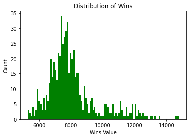
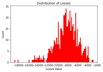
We can see wins has a right skew distribution with a small number of subjects with wins above 10,000. The losses is similarly distributed but with a left skew distribution. The presence of trials of length 150 in this data alongside the data of trials with length 95/100 would be partly the cause of this.

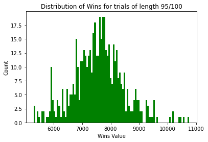
#create histogram for wins

to_keep= ['Fridberg','Horstmann','Kjome','Maia','SteingroverInPrep','Premkumar','Wood','Worthy']
filtered_df = final[final['Study'].isin(to_keep)]
plt.hist(filtered_df["tot_win"], bins=100, color="green")
plt.title("Distribution of Wins for trials of length 95/100")
plt.xlabel("Wins Value")
plt.ylabel("Count")
plt.show()

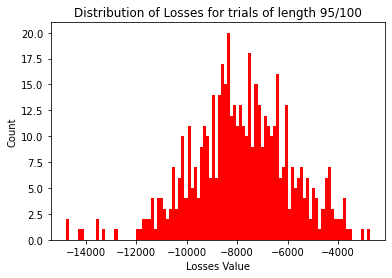
#create histogram for losses
plt.hist(filtered_df["tot_los"], bins=100, color="red")
plt.title("Distribution of Losses for trials of length 95/100")
plt.xlabel("Losses Value")
plt.ylabel("Count")
plt.show()

filtered_df.describe()

	Deck_A	Deck_B	Deck_C	Deck_D	tot_win	tot_los	Subj	Unique_ID	balance	Payoff
count	519.000000	519.000000	519.000000	519.000000	519.000000	519.000000	519.000000	519.000000	519.000000	519.000000
mean	15.132948	30.901734	23.354528	30.466281	7575.211946	-7832.080925	245.433526	260.000000	-256.868979	2.206166
std	7.125167	13.933238	14.957389	14.430446	881.667949	1960.716200	149.256183	149.966663	1169.048170	0.715170
min	1.000000	1.000000	1.000000	1.000000	5300.000000	-14800.000000	1.000000	1.000000	-4250.000000	1.000000
25%	10.000000	22.000000	13.000000	21.000000	7045.000000	-9012.500000	115.500000	130.500000	-1032.500000	2.000000
50%	15.000000	30.000000	20.000000	28.000000	7600.000000	-7800.000000	245.000000	260.000000	-300.000000	2.000000
75%	20.000000	39.000000	28.000000	38.000000	8100.000000	-6512.500000	374.500000	389.500000	550.000000	3.000000
max	38.000000	79.000000	84.000000	92.000000	10750.000000	-2725.000000	504.000000	519.000000	3570.000000	3.000000

We can see once we remove the trials of length 150 the level of right skew in the wins histogram reduces as does the level of left skew in the losses histogram.

Analysis by Payoff¶

We now look at the distribution of the balance across the different payoff schemes.

i = 1
while i < 4:
    pay1 = final['Payoff'] == i
    temp = final[pay1]
    plt.hist(temp['balance'], bins = 100)
    plt.title("Payoff "+ str(i) + " Balance Distribution")
    plt.xlabel("Balance")
    plt.ylabel('Count')
    plt.show()
    i += 1
    temp.describe()

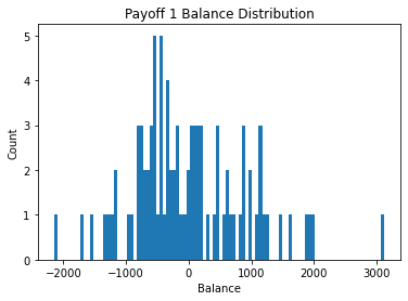
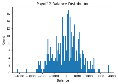
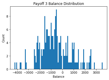
We can see payoff 2 has distribution that centers just above 0 while payoff 1 and 3 have a negative center - payoff 3 showing the worst results. This may be due to the sharp increase in penalty that occurs with every 10 cards chosen in payoff 3.

#Show wins and losses by Payoff
plt.scatter(final["Payoff"], final["tot_win"], label = "Total Wins", color="g")
plt.scatter(final["Payoff"], final["tot_los"], label = "Total Losses", color="r")

plt.legend(ncol=1, loc='upper left')
plt.title("Wins/Losses by Payoff")
plt.xlabel("Payoff")
plt.ylabel("Value")
plt.xticks([1, 2, 3])
plt.show()

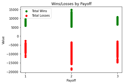
Payoff 2 shows the widest distribution across wins and losses while payoff 3 again shows a very tight distribution of wins but a wide variety of losses due to this evolving reward/punishment system every 10 cards.

Analysis by Study¶

Another theory we have is that the study in which the subject is part of may affect the participants results. We will explore this data with each study in miond to see if any obvious trends emerge. This may also be a useful clustering excercise to see if subjects will cluster with others in their study

#Show wins and losses by Study
plt.scatter(final["Study"], final["tot_win"], label = "Total Wins", color="g")
plt.scatter(final["Study"], final["tot_los"], label = "Total Losses", color="r")

plt.xticks(rotation=90)
plt.legend(ncol=2)
plt.title("Wins/Losses by Study")
plt.xlabel("Study")
plt.ylabel("Value")
plt.show()

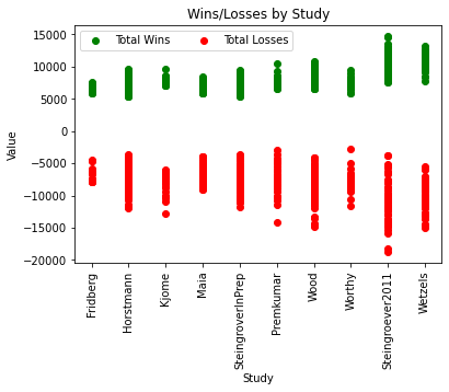
Steingroever2011 and Wetzels, as the only studies with trials of length 150, show the greatest variety in wins and losses across their participants. The Fridberg study group shows limited wins but limited losses also. This group has 15 participants so this may be a factor although Kjome shows a wider variety of wins and losses with 19 participants.

#show balance by study
plt.scatter(final["Study"], final["balance"], label = "Balance")
plt.xticks(rotation=90)
plt.legend()
plt.title("Balance by Study")
plt.show()

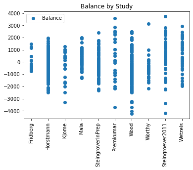
Steingroever2011, Wood and Premkumar show the widest variety in terms of positive and negative balance of its participants. Fridberg and Kjome again vary despite their similar small group size. We can also see that the two participants from Steingroever2011 which chose deck 3 150 times had the greatest profit of 3,750 amongst all participants.

Analysis of deck choices¶

One of the features we have included in our dataframe is the number of choices of each deck. We know there are good decks and bad decks with varying rewards and punishments so this will definitely be a feature that will affect our clustering algorithm.

plt.scatter(final["Unique_ID"], final['Deck_D'], label = "Deck D", s=20)
plt.scatter(final["Unique_ID"], final['Deck_C'], label = "Deck C", s=20)
plt.scatter(final["Unique_ID"], final['Deck_B'], label = "Deck B", s=20)
plt.scatter(final["Unique_ID"], final['Deck_A'], label = "Deck A", s=20)


plt.title("Deck choices by Subject")
plt.xlabel("Subjects")
plt.ylabel("Count")
plt.legend()
plt.show()

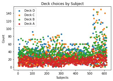
We can see above the tendency of participants to choice Decks 2/3/4 more than 60 times where deck 1 was never chosen this many times by any participant. We can also see the trend of a number of participants who have chose the same deck close to 100% of the trials. The large increase in choices from Subject 500 onwards is due to the trials of length 150.

There seems to be a unnatural distribution of choices between subjects 300-480 with a consistent number of choices being exactly 60. We will explore this data in more detail:

filter1 = final["Unique_ID"]>300
filter2 = final["Unique_ID"]<480
final_zoom = final.where(filter1&filter2, inplace=False)
plt.scatter(final_zoom["Unique_ID"], final_zoom['Deck_D'], label = "Deck D", s=30)
plt.scatter(final_zoom["Unique_ID"], final_zoom['Deck_C'], label = "Deck C", s=30)
plt.scatter(final_zoom["Unique_ID"], final_zoom['Deck_B'], label = "Deck B", s=30)
plt.scatter(final_zoom["Unique_ID"], final_zoom['Deck_A'], label = "Deck A", s=30)

plt.title("Deck choices by Subject")
plt.xlabel("Subjects")
plt.ylabel("Choice")
plt.legend()
plt.show()

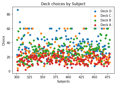
Further inspection on a subset of participants shows an unusual trend to choose a specific deck exactly 60 times. This is across decks 2/3/4 but again deck 1 is neglected in this. This may have been a stipulation of the study that no deck was allowed to be chosen more than 60 times.

plt.scatter(final["Study"], final['Deck_D'], label = "Deck D")
plt.scatter(final["Study"], final['Deck_C'], label = "Deck C")
plt.scatter(final["Study"], final['Deck_B'], label = "Deck B")
plt.scatter(final["Study"], final['Deck_A'], label = "Deck A")
plt.xticks(rotation=90)
plt.legend()
plt.title("Deck Choice by Study")
plt.xlabel("Study")
plt.ylabel("No. of Choices")
plt.show()

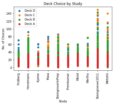
Steingroever2011 had the two most successful participants and also had the two highest choices of a single deck with two members selecting deck C 150/150 trials. There were also a number of other participants who chose a single deck more than 100 times in their study.

plt.scatter(final["Payoff"], final['Deck_D'], label = "Deck D")
plt.scatter(final["Payoff"], final['Deck_C'], label = "Deck C")
plt.scatter(final["Payoff"], final['Deck_B'], label = "Deck B")
plt.scatter(final["Payoff"], final['Deck_A'], label = "Deck A")
plt.legend()
plt.xticks([1, 2, 3])
plt.title("Deck Choice by Payoff")
plt.xlabel("Payoff")
plt.ylabel("No. of Choices")
plt.show()

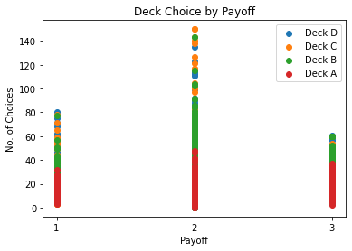
Interestingly payoff 2 shows a much higher selection of choices compared to payoff 1 or payoff 3. The distribution across these three is clearly quite different and so it will be interesting to see if clustering will indicate this also.

Introduction

Data Preprocessing, Standardization, and K-means clustering

CA4015 - Clustering Analysis of the Iowa Gambling Task

Data Cleaning¶

Importing required libraries¶

Data Import¶

Inspection of the raw data¶

Data manipulations¶

Note¶

Add Payoff to Dataframe¶

Payoff 1¶

Payoff 2¶

Payoff 3¶

Export data¶

Exploration of the data¶

Analysis by Individual¶

Analysis by Payoff¶

Analysis by Study¶

Analysis of deck choices¶